Configuring Timing In Mat Lab

Getting Started With The Siso Design Tool Matlab Simulink Example Tool Design Design History Design
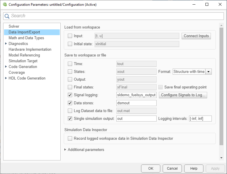
Set Model Configuration Parameters For A Model Matlab Simulink

How To Plot Real Time Temperature Graph Using Matlab Plot Graph Graphing Real Time
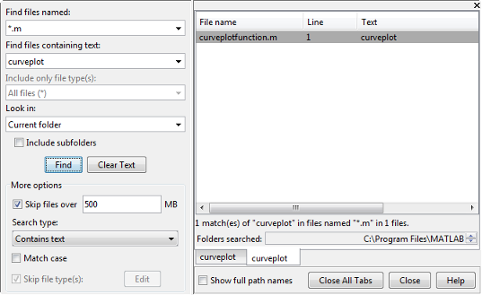
Common Errors When Calling Functions Matlab Simulink

Pid Controller Design Using Simulink Matlab Tutorial 3 Controller Design Pid Controller Control Engineering

Pid Controller Design Using Simulink Matlab Tutorial 3 Controller Design Pid Controller Control Engineering

Configuring timing parameters for can blocks the can blocks.
Configuring timing in mat lab. For more information see profile your code to improve performance. The bit rate of these four can blocks cannot be set directly. When you use the timescope object in matlab you can configure many settings and tools from the window. The text file is saved to the matlab prefdir directory.
For additional details about the performance of your code such as function call information and execution time of individual lines of code use the matlab profiler. The first step in configuring your simulation is to select a solver. Customize timescope properties and use measurement tools. Run the command by entering it in the matlab command window.
Configuring timing parameters for can blocks the can blocks. The contents of this file can be appended to a text file named javaclasspath txt.
To measure the time required to run a function use the timeit function. The bit rate of these four can blocks cannot be set directly. These sections show you how to use the time scope interface and the available tools. After you build a model in simulink you can configure the simulation to run quickly and accurately without making structural changes to the model.
Time scope uses the time span and time display offset parameters to determine the time range. Verify the matlab java path using the command javaclasspath. When you use the timescope object in matlab timescope object in matlab. To change the signal display settings select view configuration properties to bring up the configuration properties dialog box.
Configure time scope block signal display. This figure highlights the important aspects of the time scope window in matlab. Configuring timing parameters for can blocks the can blocks. By default simulink autoselects a variable step solver.
The bit rate of these four can blocks cannot be set directly. Configure time scope matlab object. You clicked a link that corresponds to this matlab command.

5 Using Matlab To Control The Motion Stage Ntu Motion Stage
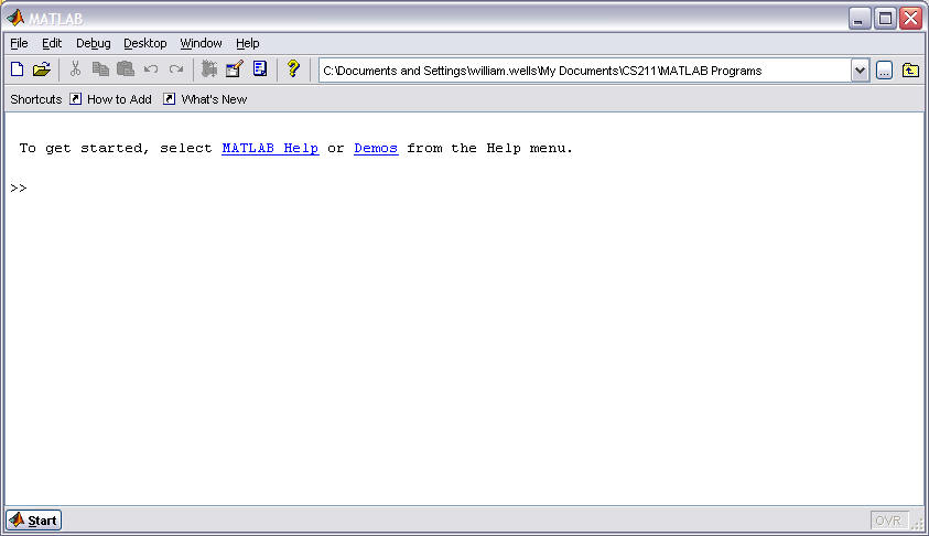
Configuring Matlab

Transfer Functions In Matlab Video Matlab

Near Field Communication Nfc Matlab Simulink Nfc Communication Systems Engineering

Display Time Domain Data Matlab Simulink

Set Breakpoints Matlab Simulink

Create A Simple Model Matlab Simulink

Continuous Time Modeling In Stateflow Matlab Simulink

Exploratory Data Analysis With Matlab Chapman Hall Crc Computer Science Data Analysis By Wendy L Martinez Chapman And Hall Crc Exploratory Data Analysis Data Analysis Computer Science

Modern Control Design With Matlab And Simulink Book By Ashish Tewari Covers Control Design Control Theory
Hydraulic Closed Loop Actuator With Fixed Step Integration Matlab Simulink Example Actuator Hydraulic Integrity

Matlab Data Logging Analysis And Visualization Plotting Dht11 Sensor Readings On Matlab Electronic Engineering Humidity Sensor Sensor

A Meme Page To Check Every Time Matlab Crashes On Twitter Visual Hierarchy Web Design Quotes Web Development Design

